Compensation Example: Step 3
Once you have all positive and negative populations defined for each of the compensation control samples, your workspace will look roughly as follows:

�At this point, it is time to bring up the compensation definition dialog window shown below, or the Compensation Wizard. The Wizard will assist you in making multiple matrices with minimum effort, and display the ancestry of your control populations for visual verification. Click here for more information.
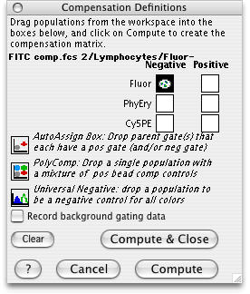
In the Compensation Definitions Dialog, select any sample with the appropriate parameters (the sample will not at this time be compensated; this selection is merely to tell FlowJo which parameters you are dealing with). For instance, you could select the first compensation sample. Then, under the Experiment menu, you will find a Compensation... menu with an associated sub-menu Define Matrix. Select this submenu, and you will be presented with a dialog window showing all parameters in the sample, and two boxes for each parameter.
Click on one of the gated populations you generated and
drag it to the appropriate box in the compensation dialog window.
For example, click on the FITC-negative population, and drag it to
the Fluor (the machine's name for FITC) box on the
left (Low). An icon appears in the box denoting that a population
has been assigned; the population's name appears above.
 �
�
If you make a mistake and drop the population into the wrong box, just select it, and press delete on the keyboard to remove it.
Continue to fill in all of the boxes for the parameters which require compensation (the scatter parameters, of course, do not require compensation in this case). In our example, all six boxes for Fluor, PhyEry (PE) and Cy5PE will have different populations. You can click on any box to check which population is being used (the name of the population appears in red near the lower left edge).
The next step is to compute the matrix and save it.
Go back to the overview of compensation.
