Compensation Example: Step 2
We must now define the populations which represent the positive (stained) and negative (nonstaining) cells for each of the singly-stained compensation samples. First of all, we will open the first sample (FITC Comp sample), in order to make a lymphocyte gate. Proper compensation requires that the positive and negative populations be gated on similar cell types (i.e., that have the same autofluorescence when unstained). Since PBMC are a mixture of monocytes and lymphocytes, which have very different autofluorescence, and the compensation stains we used only stain lymphocytes, we first make a lymphocyte gate.
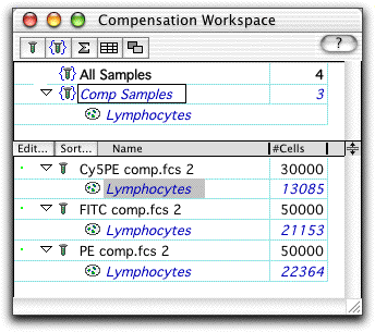
The gate was drawn around the lymphocyte population, defined by forward and side scatter. In the workspace, this resulted in the lymphocyte population being added to the sample tree.�

So that all of the compensation calculations are performed
identically, this same gate is dragged and dropped onto the Comp
Samples group, adding it to all of the compensation samples.�
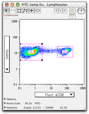
For each of the three compensation control samples, a positive and negative gate are drawn around stained and unstained cells. (Note--it is not critical that the cells be completely unstained; any two populations representing a widely disparate staining are enough.)

For simplicity, the gates are named by their stain and whether they represent stained or unstained/dim cells. In the graph above, the last population defined was the FITC-negative population, which is 36.6% of the total cells in the sample.
The next step is to bring up the compensation definition dialog window or the Compensation Wizard, and to drag the populations you just defined into the appropriate boxes.
Go back to the overview of compensation.
