Display Transformation Overview
FlowJo offers a useful technique called Transformation for visualizing compensated data without producing artifactual peaks or having cells squished against the axes.
Why change the display of your data?
When data is properly compensated, it is common that a large number of cells are displayed squished against the axis. The cells become piled up in the first channel (against the axis) because the fluorescence parameters are displayed on a log scale where it is not possible to display "zero" or negative values. The spreading of a population into negative compensated data values is the result of statistical error in measurement that is inherent in the data collected on flow cytometers. Even though the measurement error is the same in uncompensated samples, the variation becomes obvious when a compensated population has a low mean and therefore appears in the low regions of the log scale. This is because log scales expand the view of data in the lower regions (first decade) and compress the view of data in the upper regions (fourth decade). Click here for more details. FlowJo's display transformation displays your data on an altered scale that has a zero and a negative region. Note that the data is exactly the same, but FlowJo's display transform allows you to view the negative populations as nice symmetrical clusters instead of squished against the axis.
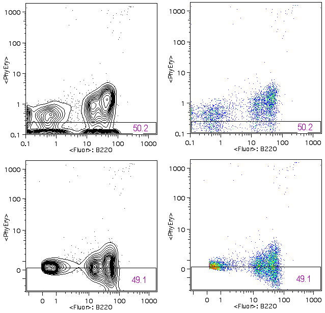
The four data plots in the figure below all show the same data. On the left two plots, the data is displayed using 5% contour plots with outliers; on the right, pseudocolor plots. All the plots show the data properly compensated. The median PE fluorescence is shown as the horizontal line on each plot . The top plots are the normal display and there are a large number of cells against the x-axis. It is worth noting that the cells against the axis are much more obvious on the contour plot.
The plots at the bottom have the display transformation applied. The cells that were squished against the axis on the top plots are now off of the axis and are shown as clusters of cells and it is now clear that the data is properly compensated. The B220 positive cell population spreads in both directions as the fluorescein fluorescence increases.

Digital Linear Data can also be transformed to provide a more interpretable view instead of the "picket fences" that occur at the low end of 5+ decade log scales.
Display transformation
Having FlowJo transform the display of your data is straightforward. After the data files have been compensated using FlowJo, select a fully-stained sample (one with some signal in all fluorescence parameters) and gate it to remove dead or unwanted cells. Select this gated population and then choose "Define Transformation..." from the Compensation menu. A custom transformation is computed based on the distribution of the data in the selected population, which results in a better visualization of your data. Click here for a more detailed description of this procedure.
NOTE: this enacts a change in display and not in your data. The compensated fluorescence values for each cell are EXACTLY THE SAME as before the transformation. The display is changed, but NOT the data. Statistics computed on a particular set of cells will be the same. The new display just makes it easier to identify correct population boundaries.
Transformation Method
The display transformation process is based on a method developed by Dave Parks and Wayne Moore at Stanford University using a generalization of the hyperbolic sine function. The display functions approach true log for high data values and approach true linear around zero. This provides smooth, near-linear display of low and negative data values.
Notes
The transformation can be used on any compensated data--but FlowJo needs to be the one to compensate the data. Therefore, it can be done on any data where you collect the comp controls and create the compensation matrix, or, alternatively, on any data files which specify their own comp matrix (currently, only BD DiVa files do this correctly).
The transformation is applied to every sample that is compensated with that compensation matrix henceforth. Therefore, if you have previously compensated data files in the workspace, the transformation will not be applied to them--UNTIL you save & close the workspace and then re-open it (at that point, all compensated files will get the transformation).
If you change the definition of a transformation for any given matrix (by selecting a different population from the original one and applying Define Transformation to it), the new transformation will automatically be applied to all samples that had the original transformation.
