tSNE
T-Distributed Stochastic Neighbor Embedding (tSNE) is an algorithm for performing dimensionality reduction: the visualization of complex multi-dimensional data in fewer dimensions that still maintain the structure of the data.
tSNE is an unsupervised nonlinear dimensionality reduction algorithm useful for visualizing high dimensional data sets in a dimension-reduced data space. In practical application using flow or mass cytometry data, the tSNE platform computes two or more new parameters from a user defined selection of cytometric parameters. The tSNE-generated parameters are optimized in such a way that observations/data points which were close to one another in the raw high dimensional data are close in the reduced data space. Importantly, tSNE can be used as a piece of many different workflows. It can be used independently to visualize an entire data file in an exploratory manner, as a preprocessing piece in anticipation of clustering, or in other related work flows. Please see the references section for more details on the tSNE algorithm and its potential applications [1, 2].
The following pages will describe and illustrate the process of running tSNE in FlowJo v9.
A use case tutorial with example data and workspace template is available. (Links to Workspace Template, FCS files, v9 tSNE Tutorial).
Practical Considerations
While tSNE is a powerful visualization technique, running the algorithm is computationally expensive, and the output is sensitive to the input data. This sections will briefly cover a few key points in the area of preparing your data.
- Cleaning up your data - The best analyses begin with cleaning up raw data to exclude doublets, debris, and dead cells. This step reduces noise in the data and can improve the tSNE algorithm output. In the tutorial workspace template, we have applied a Singlets/Lymphocytes/Live manual gating strategy to exclude doublets, debris, and dead cells respectively. In addition, gate to include only the cells of interest (e.g., gating on CD3+ if T cells are of primary interest).
- Downsampling - tSNE computation time scales exponentially with the number of input events. A Downsample Gate tool is available under the Platform menu, allowing a subset of events from a parent population to be selected and placed in a child Downsample Gate. Initiating tSNE calculation on a Downsample Gate containing 10,000 events versus 50,000, or 100,000 events, will significantly reduce calculation time. Practically speaking, the upper limit for tSNE is in the range of 100,000 events.
- Parameter Selection - In addition to choosing which events to use in your tSNE calculation, it is also important to choose appropriate parameters. If your data set is fluorescence-based, select only compensated parameters (
:Stain Reagent). Do not include parameters that may have been collected, but were not used in the staining panel, and leave out any common parameters that do not vary across the sample population you are investigating. Inclusion of irrelevant parameters can add background noise in the calculation without contributing to the signal and increase computation time. - Data Scaling - You may see an improvement in your results if your data is properly transformed and on scale. For more information on this subject, see our help pages on transformations in FlowJo v9 (links).
- Workflow - Because tSNE relies on the initial state of events seeded into the algorithm, the output will not be identical for different samples. One rational approach to comparing multiple samples is to concatenate all samples together, creating a new keyword-based parameter denoting the differences between different samples such as disease state, treatment group or study arm. From this concatenated datafile, run tSNE on an appropriately gated (and downsampled) set of events. You can then use the new sample parameter created during concatenation to color or gate the displays to identify specific samples. Note that this approach is limited given the low number of events that can be fed into the algorithm. Since it is practically limited to about 100,000 events, that means if you have 50 samples, you can select only 2000 events from each.
Creating tSNE Parameters
Basic Operation:
- Within the workspace, select a desired input gate within the hierarchy of a single sample. Try starting with a low number of events by creating a Downsample Gate.
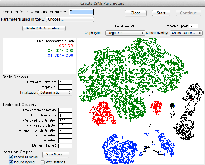
- Under the Platform menu, select Create tSNE Parameters... This will bring up a Create tSNE Parameter window with options.
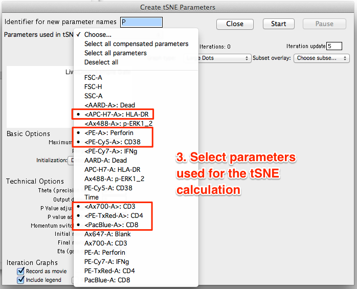
- Select the parameters to be used for the tSNE calculation. If your data is fluorescence-based, make sure to choose only compensated parameters (denoted by <parameter>).
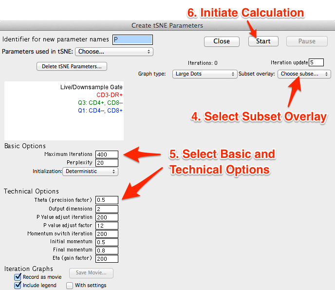
- Select gated subset(s) to overlay on the graph plot during calculation (optional). Selecting a previously gated subset downstream of the gate used to calculate tSNE will display an overlay visualizing the location of known markers within the dimension-reduced tSNE space as the algorithm runs.
- Select Basic and Technical options (optional). Defaults have been provided as a starting point and should be acceptable for most data sets. However, users may need to explore varying these options to produce a good output. Below, we modified the Basic Options defaults, setting Maximum Iterations to 400, Perplexity to 20, and leaving Initialization as Deterministic. Users are urged to read below and refer to the references section for further reading on the technical options.
- Initiate the calculation by pressing the start button.
The algorithm will run on the input population selected, utilizing selected options. The Platform will create new parameters, which are the dimension-reduced outputs from the algorithm.
Note: The parameters are named in the following fashion: "tSNE base n/m", where "base" is the identifier entered by the user in the interface (default = "P") "m" is the number of dimensions being reduced to (typically, 2), and "n" is the tSNE parameter. Thus, in a dimension reduction to two parameters, FlowJo will create two new parameters named "tSNE P 1/2" and "tSNE P 2/2". If reducing to three parameters, they would be named "tSNE P 1/3" etc. Different base names can be specified in order to create multiple sets of reduced dimension parameters.
Basic Options
- Maximum Iterations - Maximum number of iterations the algorithm will run. Default is 1000 and minimum number of iterations is 50.
- Perplexity - Perplexity is related to the number of nearest neighbors used in learning algorithms. In tSNE, the perplexity may be viewed as a knob that sets the number of effective nearest neighbors. Perplexity must be greater than the number of parameters used to calculate tSNE and less than 200. The most appropriate value depends on the density of your data. Generally a larger / denser dataset requires a larger perplexity.
- Initialization - Events can be fed into the algorithm either deterministically, by random seed, or user-specified seed event.
Technical Options
- Theta (precision factor) - Theta is a threshold that trades off between speed and accuracy; higher values of theta lead to faster but coarser approximation, lower values of theta lead to slower but finer approximation.
- Output dimensions - The number of output parameters created. Must be between 1 and the number of parameters used for the tSNE calculation.
- P Value adjust iteration - The iteration at which the tSNE probability value is modified to its final value.
- P value adjust factor - The probability value used in the tSNE algorithm is much higher during initial iterations to allow the algorithm more flexibility to move events around. Once the p value is adjusted, event movement is more constrained.
- Momentum switch iteration - The iteration upon which Momentum term changes from Initial momentum to Final momentum values.
- Initial momentum - A momentum term used in updating the weights on gradient update. Momentum tends to keep the weight changes moving in a consistent direction. Specify a value between 0 and 1, where a larger value means gives more weight to adjustments moving in the direction of previous adjustments. In general, smaller values are preferable initially to avoid over focusing on a good solution, when a better solution is available.
- Final momentum - Specify a value between 0 and 1. In general, a larger value for final momentum, compared to initial momentum, is preferable to favor convergence.
- Eta (gain factor) - The learning rate (Eta), which controls how much the weights are adjusted at each update. In tSNE, it is a step size of gradient descent update to get minimum probability difference.
Iteration Graphs
- Record as a movie - When checked, a movie of the tSNE calculation is recorded within FlowJo. To view, click Save Movie... when the calculation is complete and save the .mov file to disk.
- Include legend - When checked, a legend displaying overlaid population names will be included in the recorded movie.
- With settings - When checked, basic and technical options will be included in the movie legend.
Additional Options
- Graph type - Choose the type of graph plot to view in the window while calculating tSNE.
- Subset overlay - Select one or more gated populations to create a dot plot overlay and view the location of events with particular phenotypes in the graph plot while calculating tSNE.
Visualizing the tSNE Data Space
The Graph Window
When the tSNE calculation on a sample is complete, new tSNE parameters will become available within the drop down parameter list of the graph window. The tSNE parameters can be used in any graphic, gating, or other analysis, as can any of the original sample parameters. A gate created on the tSNE parameters should only be done as a subset of the original gate used to create the parameters. If you move any gates that change the events in that gate, the tSNE parameters will NOT be automatically recomputed.
IMPORTANT NOTE: the tSNE platform only assigns values for the created parameters for the events used in the calculation. All other events in the sample are assigned values of zero. Thus, one can display the tSNE parameters for other (e.g., parent) gates in the sample, but many events will be located at the bottom.
To visualize data using the tSNE parameters:
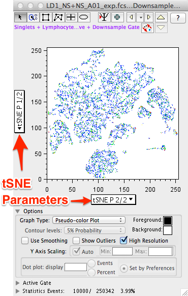
- Double click on the gated population used to calculate tSNE (in the example provided, this is a Downsample Gate containing 10,000 events). This will open a graph window.
- Select tSNE 2/2 (X-axis) vs tSNE 1/2 (Y-axis) to view the reduced data space in the same orientation as the Create tSNE Parameters window displayed during the calculation.
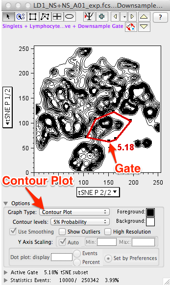
- The default plot type is (depending on your preferences) Pseudocolor. Changing the display to a Contour Plot will reveal a content-like structure with peaks and valleys representing different densities of events at the plot location.
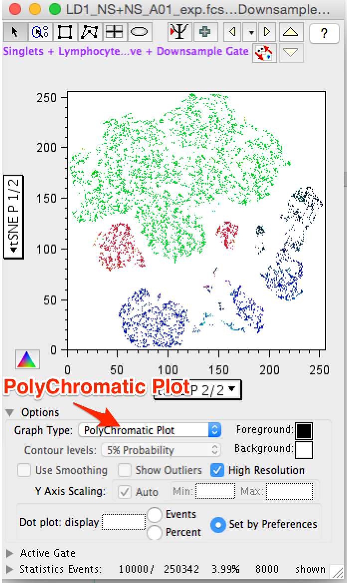
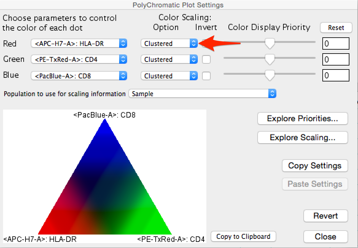
- A particularly useful plot type for exploring tSNE visualizations is the polychromatic plot. The polychromatic plot plot colors events in a plot based on the intensity of a selected parameter, or parameters. Up to three parameters can be used to create a spectrum of their interaction on any other parameters, including the tSNE parameters. Among the scaling options, 'clustered' is useful for tSNE plots as this choice will varying the coloring based on the detection of distinct clusters within the data, making these clusters stand out. In the figure below a polychromatic plot is shown on the right along with the parameter selection and color scaling pop-up menu. Note that the color triangle maps the intensity of the plotted events. In the ploychomatic plot the separation between CD4+ and CD8+ T-cells is defined by the blue and green coloring, while HLA-DR+ cells are colored red. Cells that are positive for multiple parameters color darker.
- Regardless of the plot type, gates can be drawn and subsets of events isolated based on their position within the reduced tSNE data space.
The Layout Editor
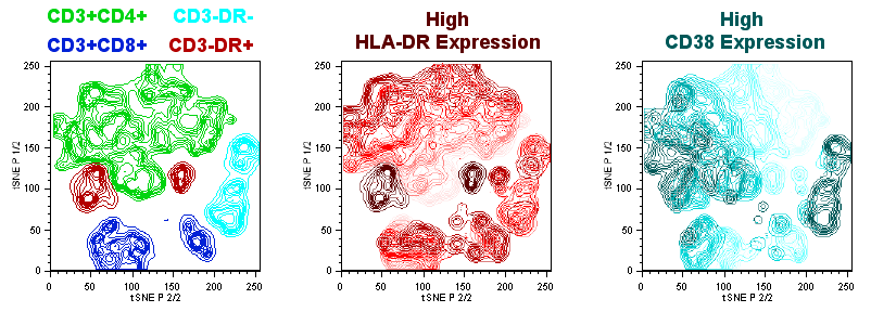
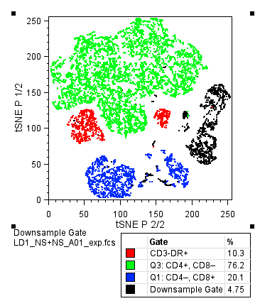
Overlays of gated populations with known phenotypes can be displayed in the dimensional reduced tSNE space using the Layout Editor, creating a graph similar to the overlay created within the Create tSNE Parameters window during calculation. In the example below, we have taken the original Downsample Gate and overlaid CD3-DR+ (red) CD3+CD4+ (green) and CD3+CD8+ (red) gated subsets. Note the distinct separation of markers in different regions of the continent structure, and the resemblance to the polychromatic plot.
Overlays representing the variation in expression of a marker can be created in the Layout Editor. Start by constructing a series of range gates on a single marker histogram profile, then overlying those populations and modifying the plot colors to illustrate graded expression pattern across the tSNE continent.