
Linear Discriminant Analysis (LDA)
LDA is an algorithm for reducing the dimensionality of a data set based on maximizing the ability to separate two or more classes within the data.
Theory
Imagine a data set as a 3-dimensional dot plot floating in the middle of your office, so that you can walk around it and look at the data from any angle you want. From some angles you will be able to distinctly visualize groups or clusters of cells separating themselves from each other. From other angles it will be harder to see those separations, but others may appear. If instead of asking you to walk around the data, we instead rotate the data and then draw a 2-dimensional representation of what we're looking at this is called projecting the data, and its what LDA does to show you the separation in a data set.
LDA creates this projection by multiplying the data by a vector that transforms it into the rotated version of itself that provides the best view of the differences in the data. There are an unlimited number of vectors that the data could be multiplied by. What differentiates one data reduction method from another is generally the criteria used to select the best vector for multiplication.
In LDA the metric is the ability to separate two or more classes of data. The goal is to find a view of the data in which different classes of data are separable by drawing a line between them. The specific statistic we use for this metric is the Variance Ratio, the result of dividing the variance within a class by the variance between classes. Returning to the 3-dimensional data example, and imagining the data plotted on an x-y-z coordinate axis, the projection created by transforming the data through LDA becomes the new x-axis. We call it LDA parameter 1, or LDA p1 for short. The vector the data was multiplied by to create LDA p1 is the first eigenvector.
The process can then be repeated to find the vector that produces the second best variance ratio, and call this vector LDA p2. The stipulation that only vectors orthogonal to the first eigenvector is used so that when we produce LDA p2, it can be plotted versus LDA p1 to create a classic 2-dimensional plot. This process can then be repeated for as many discriminant vectors as are necessary to map all of the variance between classes.
Practically, a cytometry experiment will have many more measurements made then the three in this thought experiment, so the search for the optimum eigenvectors is performed in high dimensional space using matrix algebra. Essentially each class is assumed to be normally distributed and the parameters of each distribution (means and covariance) are set up as a system of equations that can be solved for to maximizes the variance ratio. Wikipedia provides more detail if desired.
Application
In this example twelve unstimulated FCS files and 12 PMA stimulated FCS files were each gated for single cells and debris removal, then concatenated into of about 3 million events of stimulated cells, and another file of about 3 million unstimulated cells. These populations were then randomly down sampled to 1 million event subsets. By concatenating the files the LDA model can be built to closer reflect the structure of the population, as opposed to noise in an individual sample.
The LDA platform can be started by selecting one of the populations for comparison and choosing LDA from the platform menu, dimension reduction choice as shown in the figure below.
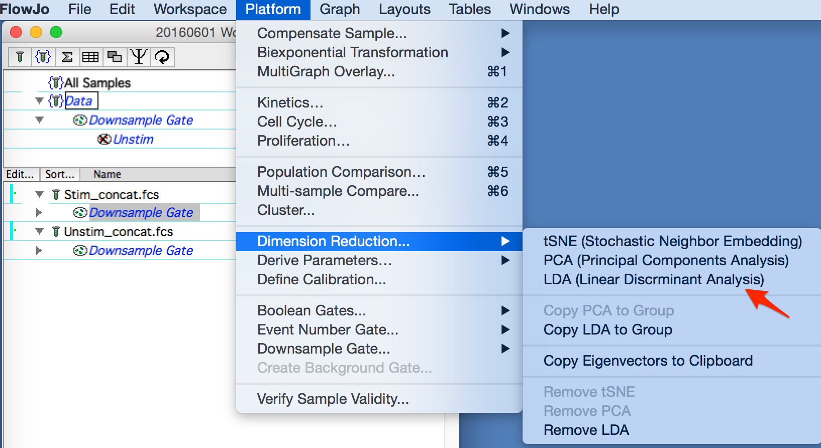
Figure 1: Starting the platform
On initial startup a red warning will display stating that a second population must be dragged in. Since LDA maximizes the variance between populations, you will need at least two populations to start.
In this example the concatenated stimulated and unstimulated populations have been dragged in for analysis, as shown in the figure below.
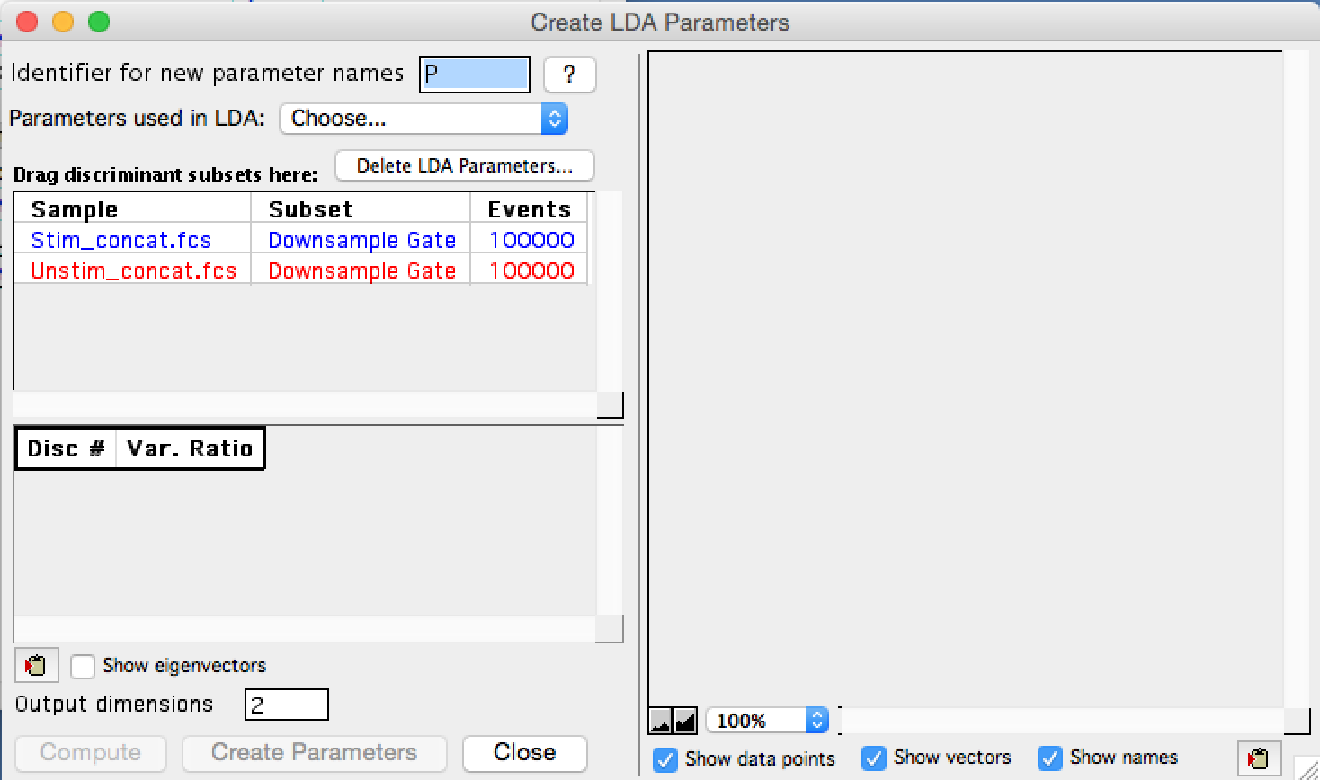
Figure 2: Two populations selected
The user can choose an identifier for new parameters; p is the default. Then to get started the parameter selector must first be used to identify which parameters are of interest. Once that has been done, the Compute button will ungray and can be clicked to start the calculation.
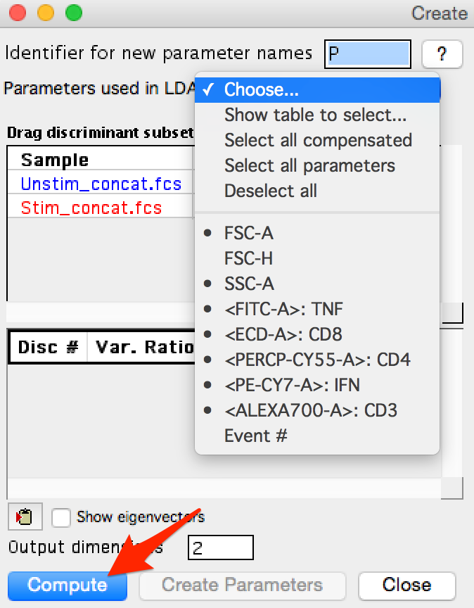
Figure 3: Parameter selection and Compute
Once the calculation completes,a plot will appear of the populations overlaid in LDA parameter space, and a table of discriminants and the variance ratio they result in is created. All discriminants are calculated on the press of compute. The 'Output Dimensions' data entry box can be used to control how many plots are made of the data, and how many parameters are created and appended to the FCS file in the workspace when 'Create Parameters' is clicked.
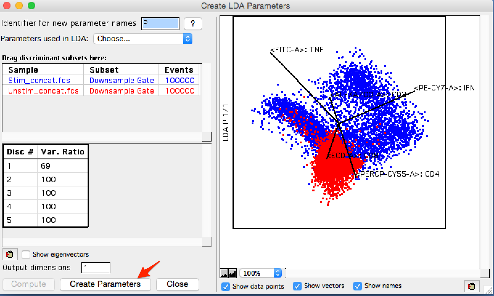
Figure 4: Results
In this example, a single parameter is enough to explain the variance between these classes, but I will choose to create 2 to create a 2-dimensional graph. At this point the LDA window can be closed and we will see the blue bar next to each incorporated sample indicating that the sample has a new derived parameter.
Use and Interpretation
To identify the populations where the unstimulated and stimulated cells different in LDA space, an overlay was created in the layout editor. In the figure below the initial plot shows the unstimulated in gray, and the stimulated overlaid and colored red. Two clear populations emerge that only contain stimulated cells, so these have been gated and just called population 1&2 to begin with. The second plot shows an overlay of these populations colored. The last two plots show each of the populations overlaid with the unstimulated file colored gray and overlaid to provide context. The green colored events express more TNF than unstimulated cells, and the blue cells are a population expressing more IFN than unstimulated cells.
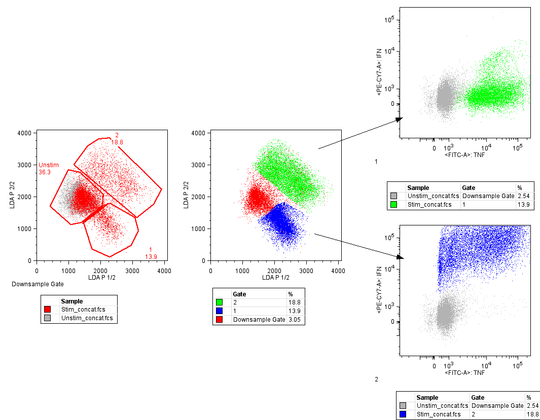
Figure 5: Data exploration