Reading FACSDiVa Data Files
Export from DiVa
BD FACS DiVaT version 4.01: - export as Experiment - This format allows for the best transformed displays of uncompensated parameters; however, very little annotation (stain names, acquisition time, etc) is included in the file. If these are important, then export as FCS 3.0, 18 bit resolution (262,144 channels). Uncompensated data will not be transformed (but compensated will be). BD recommends that you upgrade to version 4.0, and has indicated that this is a free upgrade.
BD FACS DiVaT version 4: - Export as FCS 3.0. FCS 3.0 data files from BD FACSDivaT Software v4.0 are in floating-point format and are fully annotated.
Import to FlowJo
Compensation
All data exported from the BD FACSDiVaT software (except FCS 2 files) is saved in linear, uncompensated format. If the data was compensated during acquisition, this compensation matrix is included in the data file (in FlowJo, it is referred to as the Acquisition matrix).
FlowJo will apply the Acquisition matrix to the data files. Therefore, when you add the data files to a FlowJo workspace, they show up with a red bar beside them (indicating they have been compensated). To look at the parameters uncompensated, hold the option key and click on the graph window axis pulldown lists and choose parameters without brackets <>.
The Acquisition matrix can be edited or an entirely new matrix can be created and applied to the data files. In order to replace the previous matrix, simply apply the new one to the data file. To edit the Acquisition matrix, you must first create a new matrix that is a copy of the acquisition matrix, and then edit that.
Linear or Log Scaling
Since data exported from the BD FACSDiVaT software (except FCS 2 files) is saved in linear format, the user must tell FlowJo in which format to display the data (log or linear.) The factory default FlowJo Preference is to show all fluorescence parameters in log and both side scatter and forward scatter in linear format.
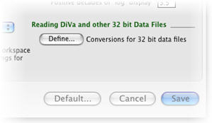
To change these Preferences, go to the menu FlowJo > Preferences. on the Workspace tab you will see Reading DiVa and other 32 bit Data Files. (Shown at right) Click on Define.
This dialog is then displayed by FlowJo:
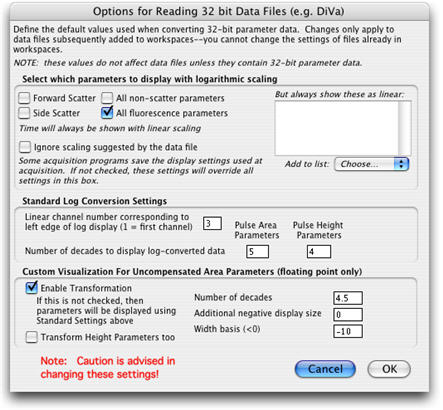
In the upper-most area, you can select which parameters should be shown with logarithmic scaling by default. In the box to the right, you can type the names of selected parameters to always display as linear (for example, when doing Cell Cycle analysis, these parameters should be linear). If you have a workspace open, then the popup menu Add to list will show parameters collected in the files in that workspace.
If you do not wish to use FlowJo's visualization aid, you can remove the check mark from Enable Transformation. You can then make your own display choices in the area called Standard Log Conversion Settings.
How Many Decades to Display
The BD FACSDiVaT software has an option to only show the top 4 decades on the plots - in order to avoid showing the picket fencing in the lower region. However, FlowJo shows all the data and transforms the way the data is displayed using Logicle scaling. This will add a small amount of negative to each axis in order to remove the picket fencing and bring the negative populations up off the axis. Note the Preference above, set to "Enable Transformation".
Display Transformation (Bi-exponential Scaling)
FlowJo can display data in order to show all the cells that are normally squished against the axis. A minor transform is applied to the uncompensated data when users export as directed above from the BD FACSDiVaT because this export generates data files that can have negative values for Area parameters. FlowJo uses a single automatic transformation for these parameters.
When you then compensate these parameters (i.e., those that are already transformed), the compensated parameters by default will get the same minor transformation. This might be enough transformation--but often isn't. For this case (and whenever you compensate data), you can still choose to create a custom transformation for your data.
For this purpose, you should select a fully-stained sample (that has fluorescence in all channels), gated to remove dead or unwanted cells (i.e., lymphocyte gate), and then choose "Define Transformation..." from the Compensation menu (under Platforms). A custom transformation is computed based on the distribution of the data, which results in a better visualization.
The custom transformation will be applied to all samples that are compensated the same way in the workspace; hence it only need be computed once for each unique compensation matrix. The transformation can be re-calculated based on a different stained sample (or gate) if necessary.
Note that if gates are drawn on a sample before it is transformed, then the positions of the gates should be verified. This is because the lower edges of the original gates may only extend down to small positive values (the original log scale)-after transformation, many events may be in the negative value area and thus no longer within the gate.